Quantum Computing 101: Quantum gates

To process information, a computer must be able to modify its bits (otherwise the machine wouldn't be very useful). For this purpose, computational circuits are used. Classical computer circuits consist of semiconductors and logic gates. Semiconductors are used to transport information through the circuit, while logic gates perform information manipulation, converting the digital signals coming from their inputs [1]. In classical computing, a gate implements binary operations on binary inputs, transforming zeros into ones and vice versa [2]. 

To exemplify the action of the logic gate, let us take single input gates, which can receive an input (0 or 1) and provide an output (0 or 1). In general, logic gates are defined by truth tables. The truth table corresponds to the outputs of a system for all input combinations. A single input port that takes a 0 as input and produces a 0 as output, or takes a 1 and produces a 1, accomplishes nothing – it might as well not be in the circuit. This type of operation that does not produce a result is called trivial. A gate that takes a 0 as input and outputs a 1, or takes a 1 and outputs a 0 can be useful in a circuit. In this case, we say that it performs non-trivial operations. In the example of single input ports, there is only one non-trivial Cbit logical operation, the NOT operation, which takes from 0 to 1 and from 1 to 0. 

What governs the output is a boolean function. I know the term may sound mysterious and somewhat complicated, but believe me, it's not. Think of a Boolean function as a rule for how to answer Yes/No questions (1 for Yes and 0 for No). It's that simple. As we have seen, gates are then combined into circuits and circuits into CPUs or other computing components. 

In a similar way, the quantum gates They are the basic building blocks of quantum computers and perform information manipulations. In quantum computing, the situation involving the manipulation of information is very different from the classical one, because Qbits can exist in superpositions of 0 and 1 and be entangled (I talked a little about the two concepts in first text in this series). There is another less well-known concept that is perhaps equally important for this manipulation: reversibility. In short, the quantum gates are reversible. If you decide to advance quantum computing, you will learn a lot about reversibility. For now, keep in mind that all quantum gates They come “from the factory” with an “undo” button. 

We can't talk about quantum gates without talking about matrices, and we can't talk about matrices without talking about vectors. We saw previously (introduction text e text postulates) that in the language of mechanics and quantum computing, vectors are described in a package called ket. To begin with, we will use two kets, |0> and |1>, which will replace the Qbits in the form of electrons in the states spin-up (|0>) and spin-down (|1>) . These vectors can encompass any number of numbers, so to speak. But in the case of a binary state, such as a Qbit of electrons spin up/down, they only have two. So instead of looking like towering column vectors, they're more like numbers stacked two high. For example, |0> represents the following stacking:

/ 1 \
\ 0 /

What the quantum gates do is transform these kets (column of numbers into vectors) into new kets. When this happens, we say that they have passed from one state to another. This magic happens through matrix multiplication. It is important to remember that the product of two matrices is defined only when the number of columns in the first matrix is equal to the number of rows in the second matrix. This way, you can use the definition as a guide and multiply the rows of the second matrix by the columns of the first. Figures 1 to 7 show how this process happens. 

We generally use an array to replace a quantum gate. The total size of the matrix will depend on the number of Qbits being operated. If we are dealing with the transformation of just one Qbit, the matrix will be nice and simple (2 x 2 with four elements). If we have two, three or more Qbits, the size of the matrix explodes. This is because the size of the matrix (and therefore the sophistication of the quantum gate) is defined by a decidedly exponential equation:

2ⁿ x 2ⁿ = total elements in the matrix

It is for this reason that, to maintain the didactic nature of the explanation, we limited the examples to just one Qbit.

There are different types of quantum gates, but I intend to focus on Pauli Gates and in  Hadamard gate, which are widely used in quantum computing to teach operations with logic gates as they are some of the most used. You Pauli Gates are important due to the fact that the essential properties of quantum gates result from the possibility of them being described by unitary matrices (when their inverse matrix is the same as yours transposed conjugate) who own property hermitian, exactly the characteristics of Paulis. O Hadamard gate can be used to convert the Qbit from the cluster state to the uniform superposed state. 

Pauli Gates

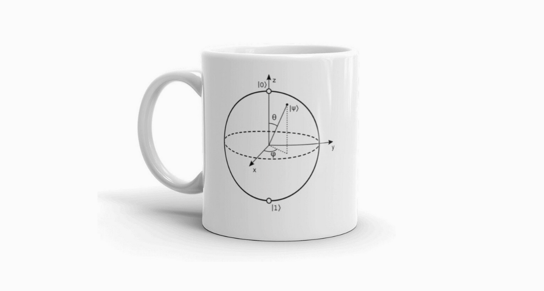
To begin with, it is worth mentioning that these doors were named in honor of the physicist Wolfgang Pauli, which was immortalized due to two of the best-known concepts in modern physics: the famous Pauli exclusion principle and the dreaded Pauli effect. The Pauli gates are based on the well-known Pauli matrices, which are incredibly useful for calculating changes in spin of a single electron. How the spin of the electron is the preferred property used to transform a Qbit into quantum gates current ones, know the Pauli matrices and their quantum gates It is extremely important for anyone who wants to manipulate quantum computers. In any case, there is essentially a gate/Pauli matrix for each axis in space (X, Y and Z), as can be seen in Figure 8.

It is important to comment that this 3D space, represented in Figure 8, is called Bloch sphere, and is the geometric place where vectors are represented [3].

The first Pauli gate What we will see is the Pauli-X gate. It represents the classic NOT gate, responsible for the negation operation. In a quantum computing circuit configuration, the X-gate is generally used to transform the state of spin-up |0> of an electron in a state of spin-down |1> and vice versa (Figure 9).

A capital “X” usually represents the Pauli-X gate or the array itself and looks like the following stackup:

/ 0 1 \
\ 1 0 /

The operation represented in ket:

|0> --> |1> OR |1> --> |0>

In terms of proper notation, applying a quantum gate a Qbit is the operation of multiplying a ket vector by a matrix. In this case, we multiply the vector ket spin-up |0> by X-gate. This way, we obtain X|0> as:

/ 0 1 \ /1\
\ 1 0 / \0/

Note that the array is placed to the left of the ket. Applying matrix multiplication, as we saw in Figures 1 to 7, and keeping the order of the elements in mind, the complete notation for applying X-gate to our Qbit (the state of spin-up of an electron), will be:

X|0> = / 0 1 \ /1\ = /0\ = |1> \ 1 0 / \0/ \1/

Applied to a vector spin-down, the complete notation would be as follows:

X|1> = / 0 1 \ /0\ = /1\ = |0> \ 1 0 / \1/ \0/

What we have in both cases is a Qbit, in the form of a single electron, passing through a quantum gate and coming out the other side with your spin completely reversed.

Let's now look at the Gates Pauli Y e Pauli Z. I'll spare you the math on these two, but I'd like you to know at least the following:

Pauli-X = [0 1] [1 0] Pauli-Y = [0 -i] [i 0] Pauli-Z = [1 0] [0 -1]

Which means that while the Pauli-X is a NOT gate, O Pauli-Y is a NOT gate with i multiple (i is the imaginary number which insanely represents the square root of -1) and the Pauli-Z inverts the sign of the second entangled state. O Pauli-Y looks a lot like the X–gate, but with an i in place of the normal 1 and a negative sign in the upper right corner. In terms of stacking, Y would be:

/ 0 -i \ \ i 0 /

O Pauli-Z is easier to understand, since it looks like the mirror image of the X–gate, but with a negative sign in the second 1. This way, Z is represented:

/ 1  0 \
\ 0 -1 /

Both (Pauli-Y e Pauli-Z) change the spin of our electron Qbit. As Pauli-Y, we have:

As Pauli-Z, we have:

Hadamard gate

While in some aspects the Pauli Gates are very similar to classical logic gates, which Hadamard gate, or H-gate, is a true quantum monster. No wonder it appears everywhere in quantum computing. O Hadamard gate has the ability to transform a defined quantum state, such as spin-up, in an obscure state, like a superposition of spin-up e spin-down at the same time. Once we send an electron spin-up or spin-down Through a H-gate, its behavior becomes similar to a coin flipping heads and tails, with a 50% chance of ending heads (spin-up) or crown (spin-down) when measured. That H-gate is extremely useful for performing the first computation in quantum programming, because it transforms predefined or initialized Qbits back to their natural state. Figure 10 shows the process visually:

In terms of matrix, we have the following representation: 

For example, when we apply the H-gate to our ket vectors spin-up |0> and ket spin-down |1>, we generate the kets |+⟩ and |-⟩:

As I mentioned, there are others quantum gates (list in English, here). Just as we can perform any classical computation with a combination of NOT + OR = NOR gates or NOT + AND = NAND gates, it is possible to reduce the list of quantum gates to a simple set of quantum gates universal. On this subject, I leave the link to a text of Scott Aaronson about. It is important to note that for a set of quantum gates To be considered universal, it must be used to perform any unitary transformation on any number of Qbits, with any desired precision. Explain, Qbits can also be used as a precise quantification metric. If the set of quantum gates can be used to approximate an arbitrary unit to any desired precision, it can be considered universal.

References

[1] Nielsen, M., and Chuang, I. Quantum Computation and Quantum Information, Cambridge University Press, 2000.
[2] Bais, F. Alexander, and Farmer, J. Doyne. The Physics of Information. Philosophy of Information, Elsevier, 2008, p. 609–83. 
[3] Carvalho, LM, Lavor, C., Motta, VS Mathematical Characterization and Visualization of the Bloch Sphere: Tools for Quantum Computing. Trends in Computational and Applied Mathematics, vol. 8, no 3, June 2007, p. 351–60. tema.sbmac.org.br, https://doi.org/10.5540/tema.2007.08.03.0351.